SOME BASIC FUNCTIONS

TABLE 1

• SUM

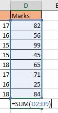
It is used for performing sum operation on the data. It can take ‘n’ number of arguments in the form of numbers.

1. For using any function, you need to first use “=” sign & then write sum (you will see the options coming), select it
   
   
   

   
2. Now select the column you want to perform operation on. (here it is Marks)

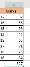
3. Press Enter & you will get the desired output

      OUTPUT

AVERAGE

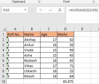
Average Function is used to calculate averages.

Steps are same to evaluate any function. It can take ‘n’ number of arguments. It is calculated as follows.

The formula is “ =AVERAGE(D2:D9) “

D2:D9 is the range of which you want to calculate average of.

• COUNT

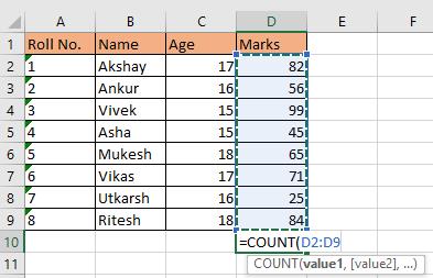
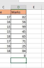
Count function is used to calculate no. of entries in the table. It cannot count strings and blanks.

For example, you want to calculate the number of values in TABLE 1 in column D i.e.

Marks

OUTPUT

• COUNTA

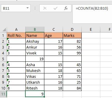
It is used to count string as well as numeric values.

The formula is “ =COUNTA(B2:B10), B2:B10 is the selected range.

As u can see it is counting strings as well as numeric values.

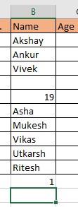
Likewise, we have COUNTBLANK. It is used to count blanks.

There is one blank in column B therefore it shows 1.

OUTPUT

• MAX

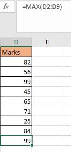
It is used to get the maximum value out of all the values. The formula is “ =MAX(D2:D9)”, where the range D2:D9 is the selected range and the highest value from it is 99.

• MIN

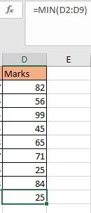
It is used to get the minimum value out of all the values. The formula is “ =MIN(D2:D9)”, where the range D2:D9 is the selected range and the highest value from it is 25.